Although Weber’s law is the most firmly established regularity in sensation, no principled way has been identified to choose between its many proposed explanations. We investigated Weber’s law by training rats to discriminate the relative intensity of sounds at the two ears at various absolute levels. These experiments revealed the existence of a psychophysical regularity, which we term time–intensity equivalence in discrimination (TIED), describing how reaction times change as a function of absolute level. The TIED enables the mathematical specification of the computational basis of Weber’s law, placing strict requirements on how stimulus intensity is encoded in the stochastic activity of sensory neurons and revealing that discriminative choices must be based on bounded exact accumulation of evidence. We further demonstrate that this mechanism is not only necessary for the TIED to hold but is also sufficient to provide a virtually complete quantitative description of the behavior of the rats.
This is a preview of subscription content, access via your institution
Access Nature and 54 other Nature Portfolio journals
Get Nature+, our best-value online-access subscription
cancel any time
Subscribe to this journal
Receive 12 print issues and online access
206,07 € per year
only 17,17 € per issue
Buy this article
Prices may be subject to local taxes which are calculated during checkout
All data are available from the authors upon reasonable request.
The custom Matlab scripts used to analyze the data are available upon reasonable request.
The authors thank D. Reato, J. de la Rocha, G. Agarwal, E. Lottem, A. Nevado, J. Paton and L. Petreanu for careful reading of the manuscript. They also thank P. Simen for pointing out relevant references, T. Stensola for help with behavioral boxes, the vivarium platform at Champalimaud Research for support, M. Bayonas for help with headphone prototyping and D. Kobak for reading the manuscript and advice on statistical analyses. J.L.P.-V. was supported by the HFSP postdoctoral scholarship LT 000442/2012, and J.R.C.-S., M.V., T.C., M.I.V. and A.G.M. were supported by doctoral fellowships from the Fundação para a Ciência e a Tecnologia. Z.F.M. was supported by the Champalimaud Foundation, the European Research Council (Advanced Investigator grant 250334), the Human Frontier Science Program (grant RGP0027/2010) and the Simons Foundation (grant 325057). A.R. was supported by the Champalimaud Foundation, a Marie Curie Career Integration grant (PCIG11-GA-2012-322339), the HFSP Young Investigator Award RGY0089 and the EU FP7 grant ICT-2011-9-600925 (NeuroSeeker).
J.L.P.-V. and A.R. conceived the project. J.L.P.-V. and M.V. conducted the rat auditory experiments. I.D., M.V. and J.R.C.-S. conducted the human auditory experiments. M.I.V., A.G.M. and Z.F.M. conducted the rat olfactory experiments. A.R., J.R.C.-S. and T.C. conceived the theory. J.R.C.-S., J.L.P.-V., M.V. and A.R. analyzed the data. A.R. wrote the manuscript with feedback from all the authors.
The authors declare no competing interests.
Publisher’s note: Springer Nature remains neutral with regard to jurisdictional claims in published maps and institutional affiliations.
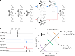
(a) Headphones used for stimulus delivery, and base (bottom). The base is chronically implanted to the skull of the animals and contains a strong miniature magnet which both holds the speakers in place during task performance and also allows easy attachment/detachment. The actual positioning of the speakers was adjusted under anesthesia to match the position of the pinnae for each rat individually relative to the base. The red material in the picture is a moldable glue (Sugru) used for strengthening the headphone structure. (b) Measurements of the acoustic shadow generated by the head. Broadband noise stimuli were played at 65, 70 and 75 dB SPL and sound level was measured placing the microphone by the ear canal of the ‘far’ ear. (c) The head plus near field positioning of the speakers causes an attenuation of 22 dB. (d) Because the head attenuation is not infinite, the sound at each ear contains a contribution from the intensity of both speakers. Thus, the intended (using the sound intensity only from the near speaker) and actual experienced intensity at each ear are not identical. We calculated the difference between the actual and experienced intensity assuming additivity of the squared pressure RMS from each speaker, and we used this to compute the difference between actual and intended ILD and ABL, which are shown in panel (d) as a function of intended ILD. Since these differences are always less than 0.1 dB (which is less than an order of magnitude smaller than the just noticeable difference (JND) for ILD of our animals) we have, for simplicity, ignored the difference between actual and intended levels throughout this study.
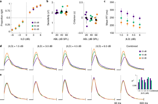
(a) Each plot shows the cumulative distribution of RTs for a given difficulty (absolute value of ILD) for the three ABLs (RTs merged across rats). The shape of the distribution for the shorter RTs is the same across all conditions. This is presumably due to the fact that sound onset after central-port entry was to some extent predictable (fixation period was drawn from a uniform distribution between 300 and 350 ms) and to the fact that we did not impose a minimum RT. These short, condition-independent RTs are thus the result of anticipation. (b) To detect the earliest time where RTs become condition-dependent, we run a two tailed Kolmogorov-Smirnoff test comparing the RTs for the fastest and slowest conditions (|ILD| = 6 dB and ABL = 60 dB SPL versus (|ILD| = 1.5 dB and ABL = 20 dB SPL) as a function of the maximum RT included in the comparison. This panel shows the p-value of the test. We defined RTmin as the value at which this comparison becomes significant (90 ms, p<0.05). This value is shown as a dashed vertical line in (a) and (c). Since we are interested in the stimulus-dependence of RTs, we excluded from all analyses RTs smaller than RTmin. (c) Same as (a) but comparing the cumulative RTDs across ILDs for each ABL separately. As expected, the distributions start to diverge later for fainter sounds. However, it is obvious that this unspecific intensity-dependent delay cannot account for the changes in the RTD as a function of ABL shown in (a). None of our results changes qualitatively if we define a separate RTmin for each ABL.
When two distributions in time are related to each other through a rigid stretching of the time axis, their percentiles are proportional. To see this, assume that distribution ρ’(t) is obtained from ρ(t) by stretching of the time axis by a factor α, so that ρ(t) = α ρ’ (αt). It follows that. \(\mathop \limits_0^\tau dt\rho \left( t \right) = \alpha \mathop \limits_0^\tau dt\rho \prime \left( \right) = \mathop \limits_0^ dt\prime \rho \prime \left(
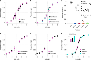
Same format as Fig. 2 of the main text. (a) Psychometric functions (n = 9 human subjects; circles, across-subject mean; lines, across-subjects standard deviation). (b) Discriminability index (left) and criterion (right) for each subject. (c) Chronometric functions ((n = 9; circles, across-subject mean; lines, across-subjects SEM). (d) RTDs for each ILD and for all ILDs combined. (e) Same but with green RTD rescaled (as explained in Methods, Supplementary Fig. 3) to maximize overlap with the orange RTD. (inset) Fraction of variance of the RTD at one ABL explained by the RTD at the other ABL (see Methods). In all panels, green (orange) corresponds to ABL = 40 (60) dB SPL. See Methods for details of the behavioral task.
Same format as Fig. 2 of the main text. (a) Psychometric functions (n = 4 rats; circles, across-subject mean; lines, across-subjects standard deviation). (b) Discriminability index (left) and criterion (right) for each subject. (c) Chronometric functions (n = 4 rats; circles, across-subject mean; lines, across-subjects SEM). (d) RTDs for each mixture contrast and for all of them combined. (e) Same but with green RTD rescaled (as explained in Methods, Supplementary Fig. 3) to maximize overlap with the orange RTD. (inset) Fraction of variance of the RTD at one mixture contrast explained by the RTD at the other mixture contrast (see Methods). In all panels, green (orange) corresponds to an odor concentration of 10 -2 (10 -1 ) (v/v). See (Mendonça, A., et al., bioRxiv, page 501858, 2019) for details of the behavioral task.
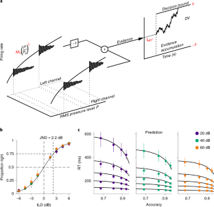
(a) In the standard use of the DDM, only the drift coefficient μ is stimulus-dependent and the variance σ 2 of the evidence is constant (Ratcliff, R. and Rouder, J., Psychological Science, 9(5):347-356, 1998; Palmer, J., et al., Journal of vision, 5(5):1-1, 2005). In contrast, if the activity of the sensory neurons is Poisson, both the mean and the variance of the evidence will in general be stimulus-dependent. In the figure, two discrimination problems (filled circles) are shown in stimulus space (s1, s2). We consider the type of stimulus dependence which holds in our experiments, \(\mu \propto s_1^\lambda - s_2^\lambda \) and \(\sigma ^2 = s_1^\lambda + s_2^\lambda \) . The difference between any two problems can be decomposed into a difference in the difficulty of the problem (gray curved lines) while keeping the variance of the evidence constant, and a difference in the effective time units of the problem (straight dark-gray lines) while keeping the intensity-ratio constant. Moving along these straight lines corresponds to a uniform stretching of the RTD; neither choice-accuracy nor the shape of the RTD (only its scale) change along this line. Moving along the equi-variance lines we change the ratio of the stimulus intensities, and thus both choice accuracy and the shape of the RTD vary. Thus, when we speak of keeping the ‘overall intensity' of the stimuli constant in the main text, we are formally referring to stimulus manipulations which keep the variance of the evidence constant. (b) In general, keeping the variance of the evidence constant while the stimuli change requires a good understanding of how the evidence relates to the stimulus. In our simple model, it requires knowing the value of λ. However, close to psychophysical threshold, keeping the variance constant is easier, since the constant σ 2 line becomes perpendicular to the identity line s1=s2. Thus, any changes which keep constant any symmetric function of the stimulus are expected to also keep the variance approximately constant. This panel shows a zoomed version of the dashed square region in (a), representing discrimination problems close to psychophysical threshold (i.e., s1 ~ s2). Gray line is as in (a), and blue line is the line representing constant ABL which we use in our experiments. Keeping s1 + s2 constant would be a worse approximation, but which would nevertheless be appropriate if s1 and s2 are sufficiently similar. (c) Here we considered whether there is anything special about the logarithmic transform. In a signal detection theory model with additive noise and a logarithmic encoding of the stimulus intensity (Fechner's model (Fechner, G., Breitkopf and Harterl, 1860)), the d’ of a discrimination is proportional to the log of the ratio of the stimulus intensities. We also obtain that the choice log-odd ratio (LOR) close to psychophysical threshold is proportional to ILD (Eq.44), i.e., the log of the ratio of the RMS pressure level of the two stimuli (Fig. 1c). However, we have not explicitly invoked a logarithmic transformation. Logarithms only appear in our description because sound level is typically measured in dB. In deriving Eq. 44, which is valid near threshold, we took the exact expression for the choice-LOR (Eq. 38) and developed it to first order in ILD. However, one can also develop this expression to first order in the small quantity 1−s1/s2. The figures shows the choice log-odds ratio (LOR) as one varies one stimulus (s1) while moving along the gray (gray line) and blue (blue and red) lines in (b). Gray is the exact LOR. Blue is the linear approximation in log s1/s2, equivalent to Eq. 44. Red is a linear approximation in (s2−s1)/s2. These two approximations are similarly accurate, at least for the range of difficulties that we have used. Thus, although the the mathematical description of our model is compact when measuring sound intensity in dB, there is nothing unique about the logarithmic transformation. For all panels in this figure, we used λ=0.1.
(a1-5) Psychometric functions. Dots are choose-right probabilities separately for each ABL (same color code as Fig. 4 main text). A single psychometric function has been fit to pooled data across ABLs (mean ± SD for each individual rat). (b1-5) The five quantiles for the RTDs for the three ABLs and their model fit. Error bars are 95% CIs across bootstrap resamples (Nr = 1000). (c1-5) RTDs for each rat and their corresponding model fit across all twelve conditions. Shaded regions represent 95% CIs across bootstrap resamples (Nr = 1000). Results are more noisy than for the pooled data but the model can still fit the behavior of each single rat accurately.
(a) Constrained fitting approach. In the main text (Fig. 4) we used a ‘constrained’ model fitting approach. For this approach, we first fit Γ~λθe from the psychometric function of the rats. Then, assuming that Γ is now fixed, we fit the remaining three parameters λ, T0, tNDT using only the two extreme values of ABL = 20 and 60 dB SPL (see Methods). The figure shows the results of this fit, which is the same data shown in Fig. 4b, c (n = 5 rats). Left: Choose-right probabilities (circles, mean ± across rats, n = 5; black line, model fit). Right: circles show the 0.1, 0.3, 0.5, 0.7 and 0.9 quantiles (mean ± SEM across rats, n = 5, black line, model fit). The variance in the shape of the observed RTDs explained by the constrained model is 97.7 ± 2.3% (see Methods, main text). (b) Unconstrained fitting approach. Alternatively, one can fit all four parameters simultaneously from all the data (RT and accuracy from all conditions, see Methods). The figure shows the results of this fitting approach in the same format as in (a). The variance in the shape of the observed RTDs explained by the unconstrained model is 98.4 ± 1.4% (c) Log parameter estimates (and JND) for the constrained (black circles) and unconstrained (white circles) models for the pooled data and for individual rats (n = 5 rats, error bar represents 95% bootstrap CI). The model fits and estimated parameter values using both model fitting approaches are almost identical. The fact that an unconstrained fit produces the same result as the constrained fit means that both the coupling between speed and accuracy as a function of ILD, as well as the effect of ABL on RTs, have the same nature in the model and in the data. Supplementary Table 3 also shows the values of the estimated parameters for both model fitting approaches using the Quantile Maximum Likelihood method (Heathcote, A. and Brown, S., Psychonomic Bulletin and Review, 11(3):577-578, 2004) (Methods), which are effectively identical to those obtained using the χ 2 Methods.
(a) We obtained an estimate of the joint probability distribution of the parameters from (unconstrained) model fits of bootstrap re-samples of our dataset. Gray: Log-parameters from 200 re-samples. Black: mean ± standard deviation across 1000 re-samples (n = 5 rats). Red dot is the fit to the actual data. There are strong correlations between λ, θe and T0. The negative correlation between λ and θe is easy to explain, since accuracy only constrains their product. The figure shows that this product (or, equivalently Γ, which sets the rat's JND) is very well specified by the data. (b) To gain an understanding of the relationship between T0 and λ we explored how they jointly determine the dependency of RT on ABL. Recall that we have assumed that RT=tNDT+τDTtθ and that this temporal rescaling relationship describes our data very accurately (Fig. 4). In order to obtain a model-independent estimate of tθ, we used a procedure analogous to the one in Supplementary Fig. 3, and inferred this estimate \(\hat t_\theta \) , linearly regressing the quantiles of the actual RT distributions for each value of ABL on those for the ABL-independent distribution of τDT specified by the dimensionless DDM in Eq. 41. We performed a single fit for all difficulties with a given ABL. Thus, we have \(\hat t_\theta \left( \right) = \left( >^2/2\lambda ^2> \right)10^< - \lambda \;ABL/20>\) which we view as a non-linear equation with ABL as the independent variable for which we have three data points per rat. Since Γ is very well specified by the data, we assume it is constant and equal to its best-fit value and consider T0 and λ as the parameters of interest. We used non-linear least squares to study how well λ and T0 are specified by this last equation. The fits were actually performed on log-parameters to avoid ambiguities due to units of measurement. The figure shows the empirical time-scale factor \(\hat t_\theta \left( \right)\) for each of the three ABL conditions and the model fits. Each color except black is for an individual rat. (c) Estimates of log T0 versus log λ from the non-linear least square fit. Colored points are estimates from bootstrap re-samples. For each color, black full circle is the mean across 1000 re-samples. Black lines represent the directions of the eigenvectors of the Fisher Information Matrix (FIM) evaluated at the best fit, with lengths proportional to the covariance of the parameters (they are not orthogonal because the x- and y-axis are stretched). Inset. The two eigenvalues of the FIM for each rat. The eigenvalues span several orders of magnitude, a signature of that the there is a ‘sloppy’ direction in parameter space in the model (the one along which log λ and log T0 are positively correlated) (Transtrum, M., et al., Physical Review E, 83(3):036701, 2011; Machta, B., et al., Science, 342(6158):604-607, 2013). Inspecting the functional form of \(\hat t_\theta \left( \right)\) , we see that its curvature with respect to ABL is determined by λ, and that λ and T0 jointly determine the overall range of \(\hat t_\theta \left( \right)\) . Sloppiness arises because similar curves can be produced by small correlated changes in curvature and range. Although curvature and range also appear correlated across rats, we believe that more rats and more values of ABL are needed to establish that this correlation is indeed a robust feature of the data. Despite sloppiness, the model is still quite sensitive to the values of \(\hat t_\theta \left( \right)\) . For instance, it is straightforward to check that the following equality should hold \(\hat t_\theta \left( \right)/\hat t_\theta \left( \right) = \hat t_\theta \left( \right)/\hat t_\theta \left( \right)\) . Artificial values of \(\hat t_\theta \left( \right)\) perfectly within the range of what we observed, but which strongly violate this equality (black circles in panel b), give poor model fits (panel b, inset).
In order to reveal the extent to which variables different from the sensory stimulus in the current trial had control over the rat's responses (Busse, L., et al., Journal of Neuroscience, 31(31):11351-11361, 2011; Fründ, I., et al., Journal of vision, 14(7):9-9, 2014), we quantified the predictive power of the history of stimuli, responses, responses after correct outcomes and responses after errors on choices in the current trial using logistic regression (n = 5 rats, see Methods). (a, b) Same data as in Fig. 5c. (a) Fraction of variance of the linear component of the logistic regression model captured by the stimulus and the four types of history effects we considered. Each dot is a single rat. Inset. Zoom in on the fraction of variance associated to the history effect predictors. (b) Area under the curve (AUC) for each rat for the actual data and for surrogate datasets where history predictors have been shuffled (see Methods). (c) Current trial stimulus predictor coefficients separately for each ILD and ABL. Coefficients are mostly ABL-independent and grow linearly with ILD. The linear increase with ILD is a signature of discriminations at psychophysical threshold (see Section 3.3 of the Supplementary Note). (d–g) Kernels for each of the four types of history predictors. Notice the difference in the scale of the y-axis between this panel and panel (c). Dots connected by lines indicate the kernel for each single rat. The larger positive-then-negative kernel in (f) (thick-line) corresponds to Rat 1, which shows a small but significant effect of history (point with relative variance > 5% in panel a, inset). This rat had a mild win-stay strategy due to a tendency to leave the back of her body aligned with the rewarded lateral port for the subsequent trial. Inset in (g) shows the basis of decaying exponentials used to express all kernels. Across the figure, error bars are bootstrap 95% CI (2000 re-samples, see Methods). These results suggest that stimulus-independent strategies have only marginal control over the responses of the rats in the task, and that their choices on a trial-by-trial basis reflect almost exclusively their perception of the ILD of the sounds in the current trial.
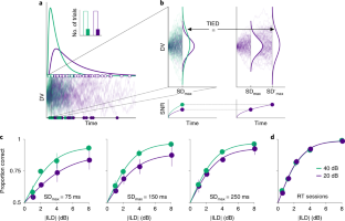
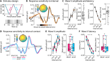
The text and mathematical details associated to this figure are in section 4 of the Supplementary Information. (a) Four representative RTDs from the drift-diffusion model. Inset. Accuracy as a function of strength of evidence. (b) Same distributions but in rescaled time. The time axis for the three slowest distributions was changed so as to maximize the overlap (minimize the Kolmogorov Smirnoff (KS) distance) with the fastest one. (c) KS distance as a function of the accuracy associated to any pair of RT distributions. (d) Same after temporal rescaling. (e) Exponential and refractory components of the RTDs shown in (a), with the same color code (see section 4 of the Supplementary Note). The refractory term (gray) is the same for all of them as it does not depend on the strength of evidence. The color lines show K(μ, σ 2 )E(t) (see Eq. 53, 54), so that the product of the two lines is the actual RTD. (f) Properties of the exponential decay term E(t) as a function of accuracy. First two lines are the mean decision-time and the time constant of the exponential decay term τExp. Third line is the strength of evidence. Fourth line is the ratio νDrift/νDiffusion (see Eq. 50) Only for accuracies very close to unity does the strength of evidence come to dominate the shape of E(t) and thus of the RTD. The different quantities in this plot are all dimensionless and have comparable values; thus we've used a single y axis whose label should be inferred from the legend. For all plots in this figure we've assumed without loss of generality that σ 2 =1.